Delayed correlation analysis (with MATLAB code)

Last time we wrote a MATLAB code for determining variances, covariances, and correlations; and then building a portfolio with optimized return to risk. The importance of correlation between different assets is the possibility of cancelling volatility in the overall value of the portfolio. The more none or negatively correlated assets you put in a portfolio, the better you can optimize it. But correlation can be used for other purposes, too.

Correlations can help us find economic cycles and impact of different markets on each other; but not the correlation that we checked before. To study the cycles and impacts we need delayed correlation analysis: impact of one move in a certain market on another one, but after a certain amount of time. A clear example, which is a common subject of many economic analyses, is the rising cycles of “inflation => interest rates => unemployment” that appear one after another!

1. To find delayed impacts, we must check correlation of the two datasets, but after adding a time delay between them;
2. To find repeating cycles in an asset, we must check correlation of its dataset against itself, but with a certain time delay.

The method explained in the second case, is also used in sound signal processing, for finding echoes, which is, by definition, a repeating sequence. So this time I wrote a MATLAB code that checks the correlation between time series of different assets (and with themselves, too) with an increasing time delay. In the end, we will plot the graph of the correlation versus the time delay. This graph will help us find out if there is a meaningful trend in the correlation, hence a delayed impact or repeating cycle (The code is pasted to the end of this post.)

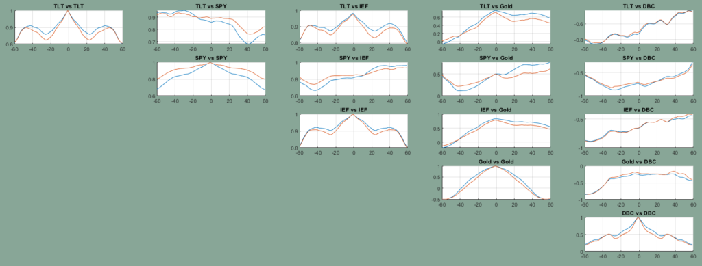
The below figure illustrates the outcome. The blue curves are the normal prices and red ones are logarithmic scales; no significant difference between them, as the first conclusion. The figure shows how correlation changes as we shift two datasets against each other with steps equal to one months. As an example, in the curve on the top-left we observe that with around -50 months delay (~4 years), the correlation between long-term bonds (TLT) and commodities index (DBC) gets very close to -1. Regarding Gold and S&P500 (SPY), we observe close to +1 correlation with the 3-4 years delay.

Another insight is the ~4-year periodic peaks on “TLT vs TLT” or “IEF vs IEF” curves. These periodic rise and falls can indicate cycles in an asset. To find these kinds of cycles, a much longer period of data and higher time frame could be better.

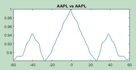
The following figure shows a ~3.5-year periodic cycle in Apple stock price. Not all assets have these kinds of periodic behavior, e.g., Gold or AMD prices.

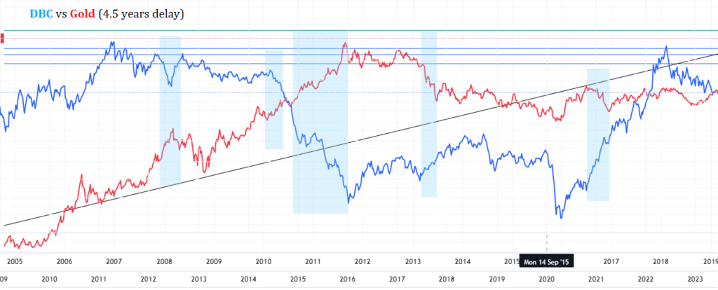
Going back to the delayed correlation between different assets, lets check the “Gold vs DBC” curve in the first figure. It shows that for a delay of around 4 years, the correlation is around -0.8, while the rest of the curve shows correlation of around -0.3 between the two assets. It means any the trend that happens in Gold today, will happen to DBC (commodities) in 3-4 years in the reverse direction. I have put their price charts (from TradingView) together with a ~4-year time shift between them, in the figure below. The wide turquoise region, as an example, marks the 2010-2011 bullish trend of Gold. Confirming the the delay correlation that we detected before, a bearish trend happened to DBC around 4 years later, on 2015-2016.

Not all delayed correlations we find in the curves above are necessarily a valid conclusion, and even if they were, finding the fundamental logic behind them could be pretty difficult. But for the sake of making it clear why this -0.8 delayed correlation shows up in this specific case, I marked several “4-years-delayed reverse trends” between Gold and DBC with the turquoise regions in the figure below.

Here is the MATLAB script for plotting all those curves. the historic prices are stored in a Data2.mat file, including a variable called “data”. Each row indicates an asset and each column is the close price of a day. Here I am using the “corrcoef” predefined MATLAB function to get correlation of historical datasets.

load Data2
assets = ["TLT","SPY","IEF","Gold","DBC"];

% preprocessing
n_assets = size(data,1);
data_length = size(data,2);


% looping through time delta
n_delta = 12*10; % 12 months of a year * 10 years
delta_unit = 22; % 22 days in a month
correls = zeros(n_assets, n_assets, n_delta-1); %preallocating the array
for n = 1:n_assets
    for m = 1:n_assets
%          if (m < n), continue, end
        for d = 1:n_delta
            if d < n_delta / 2
                dx = n_delta / 2 - d;
                temp = corrcoef([data(n, 1:data_length - dx * delta_unit); data(m, dx * delta_unit + 1:data_length)]');
                correls(n, m, d) = temp(1,2);
            else
                dx = d - n_delta/2;
                temp = corrcoef([data(m, 1:data_length - dx * delta_unit); data(n, dx * delta_unit + 1:data_length)]');
                correls(n, m, d) = temp(1,2);
            end
        end
    end
end


% plotting the outcome
for n = 1:n_assets
    for m = 1:n_assets
        if (m < n || n == m*100), continue, end
        subplot(n_assets,n_assets,m+(n-1)*n_assets);
        hold;
        plot(-n_delta/2:n_delta/2-1,reshape(correls(n,m,:),1, []), "DisplayName",assets(n) + " " + assets(m));
        title(assets(n) + " vs " + assets(m));
        grid on;
        hold;
    end
end